Some common, everyday types of measurements are:
- counting
- length
- area
- volume
- mass
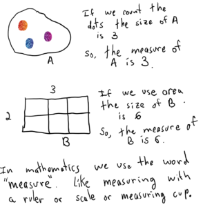
Example. The counting measure m counts how many elements are in set. So, if A is a set, then  = |A|")

We can count A and B separately (above, left) and then add the results; or we can count A and B together (above, right), either way we get the same answer (5). The above Figure also illustrates the Corollary to the Counting Theorem.
In mathematics, the idea of a measure, is abstracted into the following definition.
We say that m measures the subsets of S if m satisfies the following two rules:
- If
then
. In other words m is non negative.
- If A and B are disjoint subsets of S then
.
Proposition 1. The measure of the empty set is always 0. In other words:
 = 0")
Click here for proof of Proposition 1.
Proposition 2: Suppose that A and B are subsets of S and that A is contained in B then
 \leq m(B)")
Click here for proof of Proposition 2.
Proposition 3. If  \leq m(S)")
Click here for proof of Proposition 3.
Probability
Definition. P is probability on the subsets of S if P is a measure on the subsets of S and P(S) = 1.
Since probability is a measure, like counting, area or volume, etc., you can use your intuition about measuring to help you understand probability. However, unlike counting, area, or volume, the maximum probability is 1. An additional Intuitive way to thing about probability is to imagine it being a ratio, like shown in the picture below.

Propositions 1, 2, and 3, about measures imply the following.
If P is a probability on the subsets of S then:
- If
.
.
- If A and B are disjoint subsets of S then
.
Probability terminology
In probability you have a process (for example you toss a coin) which has a set of possible outcomes S (the coin lands heads or tails, so S = { H, T } ).
When talking about probability the set S is called the “set of all possible outcomes“; the subsets of S are called events. The probability of an event is always between 0 and 1. If the probability of an event is close to zero, it rarely will happen. If the probability of an event is close to 1, it happens most of the time.
Interpretations of probability
a philosophical note
The frequentist interpretation of probability views probability as telling you at what relative frequency an event will happen: if you toss a coin, the probability of heads is 1/2 because if you toss a coin over and over, you typically get heads about 1/2 the time. The frequentist approach places probability within empiricism: empiricism is the philosophy which emphasizes the role of experience and experiments to understand the world.
The classical interpretation of probability views probability as arising from some sort of symmetry in the possible outcomes: if you toss a coin, the probability of heads is 1/2 because if you toss a coin, there are only two possible outcomes, heads or tails, both equally likely (symmetry), so the probability of heads is 1/2. The classical approach places probability within rationalism: rationalism is the philosophy which emphasizes the role of “thinking” and “imagining”, especially logical, rational thinking in understanding the world.
There are other interpretations of probability. For more information see Wikipedia:
https://en.wikipedia.org/wiki/Probability_interpretations
Turning a finite measure into a probability
If m is any finite measure on S, meaning that m(S) is not infinite, we can turn m into a probability measure P on S if we define P as follows: for each  = \dfrac{m(A)}{m(S)}")
Equally likely outcomes
(the discrete uniform distribution)

The probability of A is basically how big A is relative to S. In other words,
If S is set and we want each element of S to be equally likely, we can define P as follows.
Let m be the counting measure on S and define the (equally likely) probability P on S as:
This probability gives rise to the discrete uniform distribution. when we learn about random variables and distributions we will revisit this example.
Example 1. Suppose S = {1, 2, 3, 4, 5 }. To define the equally likely probability on S we let m be the counting measure on S, Then, for each
Example 1 continued. Suppose A = {1, 2, 3}. Then  = \dfrac{m(A)}{m(S)} = \dfrac{3}{5}")
Example 2:
Question. Suppose I randomly pick a number between 1 and 5. Find the probability that the number I picked was even.
Answer. Let S = { 1, 2, 3, 4, 5}; E = the even numbers between 1 and 5 = {2, 4}; m = the counting measure, so  = |E| = 2")
 = |S| = 5")
 = \dfrac{m(E)}{m(S)} = \dfrac{2}{5}")
Dice Rolling
Dice provide many excellent probability examples. For information about dice see Wikipedia: https://en.wikipedia.org/wiki/Dice
Interesting note. Die is the singular of dice. One die, two dice.
If you roll a pair of die there are 36 possible outcomes because 6 x 6 = 36, for details, see the following Figure.

Let S = set of all possible outcome (rolls) if we roll a pair of dice. So, using the notation from the above Figure, we have:
S = {(1,1), (1, 2), . . . , (6, 5), (6, 6)}.
|S| = 36 = 6 x 6.
Each roll is equally likely. So, let P be the equally likely probability on S.
So P(any particular role) = 1/36
When we roll a pair of dice we usually are interested in what the roll sums to. So, we might say, “what is the probability of rolling a 7” when we what we mean is, “what is the probability of getting a role that sums to 7”.
We can easily calculate the following probabilities for a pair of dice.
P(roll sums to 2) = 1/36 because there is only one role that sums to 2, we need to get (1, 1)
P(roll sums to 3) = 2/36 because there are two rolls that sum to 3, the rolls (1,2) or (2, 1)
Etc.
We get the easy to remember probability rule for rolling a pair of dice.
(I’ll just write “roll” instead of “role sums to” to save space.)
P(roll 2) = 1/36 = P(roll 12)
P(roll 3) = 2/36 = P(roll 11)
P(roll 4) = 3/36 = P(roll 10)
P(roll 5) = 4/36 = P(roll 9)
P(roll 6) = 5/36 = P(roll 8)
P(roll 7) = 6/36
Question: What is the probability if you a roll a pair of dice of that the roll sums to 11 or 12?
Answer: P(roll 11 or 12) = P(roll 11) + P(roll 12) = 2/36 + 1/36 = 3/36
Question: What is the probability if you a roll a pair of dice that the roll will sum to less than 7?
Answer:
P(roll less than 7) = P(roll 2) + P(roll 3) + P(roll 4) + P(roll 5) + P(roll 6)
= 1/36 + 2/36 + 3/36 + 4/36 + 5/36
= 15/36
Question: What is the probability if you a roll a pair of dice that the roll will sum to 7 or more?
Answer: We can use the complement principle to easily solve this.
P(roll 7 or more) = 36/36 – 15/36 = 21/36
The complement principle
Many problems in probability are easily solved using the complement principle, which is just a fancy way of saying that:
P(A) + P(complement of A) = 1
Question: If the probability of A is 1/3 what is the probability of the complement of A?
Answer: Using the complement principle we have:
P(A) + P(complement of A) = 1
1/3 + P(complement of A) = 1
P(complement of A) = 1 – 1/3 = 2/3