The following 5 videos (run times are from about 5 to 8 minutes each) will help you with your Blackboard homework on this unit.
Please scroll down past these homework videos for an in-depth explanation of the t-distribution and confidence intervals for the mean.
Confidence Intervals for the mean
For other videos, see the video a few paragraphs down and the video solution to Question 11 at the bottom of this page
Suppose we want to know the average weight of cherry tomatoes. Not just of the cherry tomatoes in a sample. But of all the cherry tomatoes on planet earth. We can’t weigh all the tomatoes on earth. So, instead we weigh a sample of cherry tomatoes obtained by simple random sampling. Let $x$ be the random variable that measures the weight of a cherry tomato. If the mean weight of the sample is 25 grams (so $\bar{x} = 25$ g) we would estimate that the mean weight $\mu_x$ of all the cherry tomatoes on earth is also 25 grams (point estimate of $\mu_x = 25$ g). However, unless we are very lucky, our point estimate will probably be off (wrong) by at a least a little. Moreover, a point estimate doesn’t indicate anything about the “accuracy” of the estimate.
What we can do is use statistics from the sample to calculate a confidence interval (abbreviated CI). Roughly speaking, a confidence Interval is a range of values we are fairly sure contains the true value of the parameter we are estimating. In this unit the parameter we are estimating is the population mean $\mu_x $.
Note. In a simple random sample each member of the sample is individually randomly chosen from the entire population.
Example. Suppose the size of the sample was $n = 36$ cherry tomatoes; the mean of the sample was 25 grams; and the standard deviation of the sample was 5 grams. It turns out that the the 95% confidence interval for $\mu_x$ is the interval 23.31 grams to 26.69 grams, which may also be written as $25 \pm 1.69$ grams, with the 1.69 grams being called the margin of error (MOE).
Here is a 5 minute video of how to do the above calculation.
See Parts I and II (below) for detailed explanations of confidence interval calculations.
If you are short on time, just focus on Part II.
Here is an R script to do the above calculation (without using the t-distribution look-up table).
 mean_x = 25; # mean of sample
sd_x = 5; # standard deviation of sample
n = 36;   # size of sample
CI = .95  # type of CI
#----------- No user input needed below this line ---
df = n-1;
SE = sd_x/sqrt(n);
t_star = qt( (1 - CI)/2, df, lower.tail = FALSE);
MOE = t_star * SE
LowerLimit_CI = mean_x - MOE;
UpperLimit_CI = mean_x + MOE;
n
df
SE
MOE
LowerLimit_CI
UpperLimit_CI
# End of Script
Technical interpretation of the CI. If we collected samples of size $n = 36$ cherry tomatoes over and over, and for each sample we calculated a 95% confidence interval, 95% of those confidence intervals would contain the true mean weight $\mu_x$ of all the cherry tomatoes on earth. The interval $25 \pm 1.69$ grams was the 95% confidence interval generated by our sample. It might or might not contain the true value of $\mu_x$.
Quick (fuzzy) interpretation of the CI. The margin of error in a confidence interval gives us an indication of how “accurate” we should consider our point estimate (25 g) to be.
Part I is quite technical and you can quickly skim over it.
Part II is the important part for your homework.
Part I
Confidence Interval Formula when $\mathbf{\sigma}$ is known
Suppose that $x$ has mean $\mu_x$ and standard deviation $\sigma_x$. Suppose that $\bar{x}$ is (at least approximately) normally distributed (e.g, if the CLT applies):
$$\bar{x} \sim N(\mu_{\bar{x}}, \sigma_{\bar{x}})$$
We want to find $M$ such that
$$P(\bar{x} – M < \mu_x < \bar{x} + M) = 1 – \alpha$$
typically, $\alpha = 0.05$ so that $1 – \alpha = 0.95$.
$1 – \alpha$ is almost always written as a percent, e.g., $1 – \alpha = 95\%$.
The interval
$$[\bar{x} – M , \bar{x} + M]$$
is called a $(1 – \alpha)$ confidence Interval for $\mu_x$.
Confidence intervals are usually written using the “plus or minus” symbol which is a plus sign on top of a minus sign: $\pm$
An example of how the $\pm$ symbol works:
$5 \pm 2$ gives you the numbers 5 – 2 (which is 3) and 5 +2 (which is 7).
Using the “plus or minus” notation we would write the confidence interval as
$$\bar{x} \pm M$$
M is called the margin of error. It is typically abbreviated as MOE.
“Confidence interval” is abbreviated as CI
The following calculation establishes the confidence interval formula for when $\sigma_x$ is known:
$P(\bar{x} – M < \mu_x < \bar{x} + M)$
$= P(-\mu_x – M < – \bar{x} < -\mu_x + M) $
$= P(\mu_x + M > \bar{x} > \mu_x – M) $
$= \ P(\mu_x – M < \bar{x} < \mu_x + M)$
$= P(z( \mu_x – M) < z(\bar{x} ) < z(\mu_x + M)) $
$= P\left( \dfrac{-M}{\sigma_{\bar{x} } } < z < \dfrac{M}{\sigma_{\bar{x} } }\right)$ Equation (1)
In the last equality, Equation (1) we used the $z$ transformation of $\bar{x}$, which is:
$z(\bar{x}) = \dfrac{\bar{x} – \mu_{\bar{x}}}{\sigma_{\bar{x}}} $
so:
$z(\mu_x + M) = \dfrac{\mu_x + M – \mu_{\bar{x}}}{\sigma_{\bar{x}}} = \dfrac{M}{\sigma_{\bar{x}}}$
$z(\mu_x – M) = \dfrac{\mu_x – M – \mu_{\bar{x}}}{\sigma_{\bar{x}}} = \dfrac{-M}{\sigma_{\bar{x}}}$
Before we can finish the derivation of the confidence interval formula we need to define $z_\alpha$
The $\alpha$ in $z_\alpha$ corresponds to the amount of area in the tail of the distribution. Here’s the technical definition, followed by an Example.
Let $0 < \alpha < 0.5$. We define $z_{\alpha}$ by the equation
$$P(z < -z_{\alpha}) = \alpha$$
Since $0 < \alpha < 0.5$ it is the case that $z_\alpha > 0$.
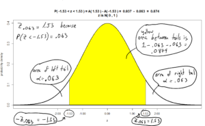
Example. $z_{.063} = 1.53$ because $A(-1.53) = .063$. See Figures below. We can find $z_{.063}$ by looking in the z-table (in the inside part) for the area closest to .063. We see that $A(-1.53) = .063$, so $z_{.063} = 1.53$ (we get rid of the negative sign).

Question 1. If $\alpha = .025$ find $z_{\alpha}$
Answer to Question 1.
$z_{.025}$ is defined by the equation
$$P(z < -z_{.025}) = .025$$
So, we look in the z-table for the z which makes $A(z) = .025$. See table below. We see that $A(-1.96) = .025$, so $z_{.025} = 1.96$ (because $ -(-1.96) = 1.96$).
Question 2. If $\alpha = .05$ find $z_{\alpha/2}$
Answer to Question 2.
Same answer as Question 1. See z-table below.
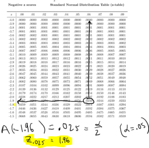
The above z-table solves questions 1 and 2.
Question 3. If $\alpha = .05$ then $z_{\alpha} = z_{.05} = 1.64$ approximately. See z-table below.

End of Question 3.
We are now ready to resume the derivation of the confidence interval formula.
By symmetry and the complement principle we have:
$$P(z < z_{\alpha} ) = 1 – \alpha$$
It follows that:
$P\left(- z_{\frac{\alpha}{2}} < z < z_{\frac{\alpha}{2}} \right) $
$ = P\left(z < z_{\frac{\alpha}{2}}\right) – P\left( z < -z_{\frac{\alpha}{2}} \right)$
$= \left(1- \dfrac{\alpha}{2}\right) – \frac{\alpha}{2}$
$= 1- \alpha$
Combining this, with Equation (1), we get
$$z_{\alpha/2} = \dfrac{M}{\sigma_{\bar{x}} }$$
and so
$$M = z_{\frac{\alpha}{2}}\, \sigma_{\bar{x}} = z_{\frac{\alpha}{2}}\, \dfrac{\sigma_x}{\sqrt{n}} $$
So, the $1 – \alpha$ confidence interval formula for $\mu_x$ with $\sigma_x$ known is:
$$\bar{x} \pm z_{\frac{\alpha}{2}}\, \dfrac{\sigma_x}{\sqrt{n}}$$
Question 4. Find 95% confident interval formula for $\mu_x$ if we know $\sigma_x$.
Answer to Question 4. Since we are finding the $1 – \alpha = 95\%$ confidence interval $\alpha = .05$ and so
$$z_{\frac{\alpha}{2}} = z_{\frac{.05}{2}} = z_{.025} = 1.96 $$
so the confidence interval formula:
$$\bar{x} \pm z_{\alpha/2}\ \dfrac{\sigma_x}{\sqrt{n}}$$
becomes:
$$95\%\ \text{CI for } \mu_x = \bar{x} \pm 1.96\ \dfrac{\sigma_x}{\sqrt{n}} \ \ (answer)$$
Note. $$P(-1.96 < z < 1.96) = 95\%$$
See Figure below.

The above Figure corresponds to Question 4.
Question 5. Let $x$ be the random variable that measures the weights of Empire apples. Suppose that we know that the standard deviation $\sigma_x = 20$ grams. If the mean weight of a sample of 100 Empire apples is 155 grams, find the 95% confidence interval for $\mu_x$.
Answer to Question 5. By the answer to Question 4 we know that the 95% confidence interval for $\mu_x$ is given by
$$95\%\ \text{CI for } \mu_x = \bar{x} \pm 1.96\ \dfrac{\sigma_x}{\sqrt{n}} $$
Substituting in $\bar{x} = 155$, $\sigma_x = 20$, and $n = 100$ we get
$$95\%\ \text{CI for } \mu_x = 155 \pm 1.96\ \dfrac{20}{\sqrt{100}} \text{g} $$
$$95\%\ \text{CI for } \mu_x = 155 \pm 3.92 \ \text{g} \ \ (answer)$$
Part II
Confidence Interval Formula when $\mathbf{\sigma}$ is unknown and the t-distribution
In real-world statistics we don’t know $\sigma_x$ and so we can’t directly use the $1 – \alpha$ confidence interval formula derived in the previous section:
$$\bar{x} \pm z_{\frac{\alpha}{2}}\, \dfrac{\sigma_x}{\sqrt{n}}$$
we have to modify it. The first modification is we approximate the population standard deviation $\sigma_x$ by the sample standard deviation $S_x$.
Recall
$$S_x = \sqrt{ \dfrac{\sum (x-\bar{x})^2}{n-1} }$$
The second modification is to use the t-distribution with n-1 degrees of freedom instead of the z-distribution.
In situations where we would use the standard normal distribution, but we can’t, because we are approximating $\sigma_x$ by $S_x$ we use a distribution called the t-distribution. The t-distribution is defined by one parameter, called its “degrees of freedom” abbreviated df. The t-distributions look almost the same as the z-distribution. Like the z-distribution, the mean, median, and mode of the t-distribution is $0$. Moreover, the PDF for the t-distribution is symmetric about 0, same like the z-distribution. The t-distribution is a little flatter than the z-distribution because of the uncertainty introduced by the approximating $\sigma_x$ by $S_x$. The Figure below compares t-distributions with with different degrees of freedom to the normal distribution.

The above Figure shows t-distributions with various degrees of freedom. The dashed line is the standard normal distribution $z$. As the degrees of freedom increases the t-distribution becomes closer and closer to the z-distribution.
With these two modifications the the formula for the $1 – \alpha$ confidence interval for the mean $\mu_x$ is:
$$ \displaystyle{\bar{x} \pm t_{\frac{\alpha}{2}, n -1} \ \frac{S_x}{\sqrt{n}}}$$
Notation. For $0 < \alpha < 0.5$ we define $ t_{\alpha, n} $ by the equation
$$P\left(t < -t_{\alpha, n} \right) = \alpha$$
where the $t$ in the above probability refers to the t-distribution with $n$ degrees of freedom.
We can have R calculate $ t_{\alpha, n} $ for us, or we can look it up in the t-distribution table.
Embedded in this page, immediately following Question 6, is the t-distribution look-up table.
Question 6. Find $t_{.025, 7}$.
Answer to Question 6.
Using R we get $t_{.025, 7} = 2.364624$
# t_alpha_n = qt(alpha,n, lower.tail = FALSE)
qt(.025,7, lower.tail = FALSE)
# End of Script

Using the t-distribution table we get $t_{.025, 7} = 2.365$
End of Question 6.
The t-distribution look-up table
Use the controls at the bottom of the embedded t-distribution look-up table
to navigate between its first and second page.
Download link is under the embedded z-table.
Note. The values we look up inside the t-distribution table, such as $t_{.025, 7}$, are often called critical values.
Notation. Often we will just write $t_*$ instead of the more complicated $t_{\frac{\alpha}{2}, n -1}$. In which case, the CI formula for $\mu_x$ is written:
$$\bar{x} \pm t_* \dfrac{S_x}{\sqrt{n}}$$
Important note. Notice, in the confidence interval formula, that as $n$ increases, the MOE decreases. In other words, everything else being equal, larger samples are more likely to give better, more “accurate” estimates for $\mu_x$.
Remember. For the CI formula for $\mu_x$ the degrees of freedom is always $n-1$.
Useful terminology and formulas for CI calculations
point estimate of $\mu_x = \bar{x}$.
standard error$ = \text{SE}\ = \dfrac{S_x}{\sqrt{n}}$
margin of error $ = $ MOE $ = t_* \ \dfrac{S_x}{\sqrt{n}}$.
Confidence Interval Questions using t-distribution
$\mathbf{\sigma_x}$ estimated by $\mathbf{S_x}$
Question 7: In a sample of $9$ black bears the mean weight was $\bar{x} = 400$ pounds and the standard deviation was $S_x = 80$ pounds. Using this data find the 95% confidence interval for the mean weight of black bears. Also find the standard error SE and the margin of error MOE. For this question assume that the weights of black bears are normally distributed. So even though the sample size is smaller than 30, the CLT applies, meaning $\bar{x}$ will be normally distributed, allowing us to use the t-distribution to find the confidence interval for $\mu_x$.
Answer to Question 7:
CI formula for $\mu_x$ is $\bar{x} \pm t_* \dfrac{S_x}{\sqrt{n}}$.
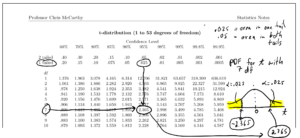
We are given $\bar{x} = 400$ and $S_x = 80$ in the problem. We only have to find $t_*$. There are $n-1 = 9-1 = 8$ degrees of freedom. So we look in the t-distribution look-up table, shown below, in the row for 8 df and in the column for the 95% Confidence Level. So $t_* = 2.306$.
We plug these into the CI formula to get the 95% CI for $\mu_x$:
$ \bar{x} \ \pm \ t_* \dfrac{S_x}{\sqrt{n}} $
$= 400 \ \pm \ 2.306 \dfrac{80}{\sqrt{9}}$
$= \underbrace{400 \ \pm \ 61.49333 \text { pounds }}_{\text{answer}}$
The $SE = \dfrac{S_x}{\sqrt{n}} = \dfrac{80}{\sqrt{9}} = 26.67$ and the
margin of error $ = t_* \dfrac{S_x}{\sqrt{n}} = 61.493.$
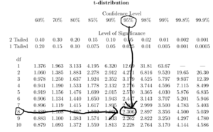
t-distribution table used to solve Question 7.
Question 8. The Eastern American Toad (Bufo a. americanus) is a smallish toad found throughout northeastern North America (including New York State). In a sample of $81$ adult female Eastern American Toads the mean weight was $\bar{x} = 43.5$ g and the standard deviation was $S_x = 15.1$ g. Using this data find the 95% confidence interval for the mean weight of adult female Eastern American Toads as a species. Use the CI formula for $\mu_x$
$$\bar{x} \pm t_* \dfrac{S_x}{\sqrt{n}}$$
Answer to Question 8. The only slightly difficult part of this problem is figuring out $t_*$. To figure out $t_*$ we look in the t-distribution table. To use the t-distribution table you need to know which row to look in and which column:
The row is the degrees of freedom (d.f.), which for the problems we’ll work on will always be $n-1$. So the d.f. $= n-1 = 81 -1 = 80$. So we look in row 80. We want the 95% confidence interval, so we look in column that says 95% confidence level. So we get $t_* = 1.990$.
Then we just plug $n = 81,\ \bar{x} = 43.5\ g; \ S_x = 15.1 \ g;$ and $t_* = 1.990$ into the CI formula:
$$CI = \bar{x} \pm t_* \frac{S_x}{\sqrt{n}}$$
which becomes:
$95\%$ CI for $\mu_x = \bar{x} \pm t_* \frac{S_x}{\sqrt{n}}$
$= 43.5 \pm 1.990 \frac{15.1}{\sqrt{81}}$
$= 43.5 \pm 1.990 \frac{15.1}{9}$
$= \underline{43.5\ g \ \pm \ 3.34 \ g}. \ \ \leftarrow$ answer.
Using the t-distribution table to find $t_*$ for Question 8.
Question 9. In a sample of $64$ adult male Eastern American Toads the mean weight was $\bar{x} = 26.3$ g and the standard deviation was $S_x = 5.0 $ g. Using this data find the 98% confidence interval for the mean weight of all adult male Eastern American Toads in the population. Use the CI formula for $\mu_x$
$\bar{x} \pm t_* \frac{S_x}{\sqrt{n}}$
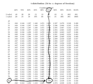
Answer to Question 9. The row is the degrees of freedom (d.f.). For confidence intervals for $\mu_x$ the df = $n-1$. So, the d.f. $= n-1 = 64 – 1 = 63$. We want the 98% confidence interval, so we look in column that says 98% confidence level. The intersection of the row for 63 d.f. and the column for 98% Confidence Level gives us $t_* = 2.387$.
Then we just plug $n = 64,\ \bar{x} = 26.3\ g; \ S_x = 5.0 \ g;$ and $t_* = 2.387$ into the CI formula.
$98\%$ CI for $\mu_x$
$= \bar{x} \pm t_* \frac{S_x}{\sqrt{n}}$
$= 26.3 \pm 2.387\ \frac{5.0}{\sqrt{64}}$
$= 26.3 \pm 2.387\ \frac{5.0}{8}$
$= \underline{26.3 \ g \ \pm 1.49 \ g}. \ \ \leftarrow$ answer.

Using the t-distribution table to find $t_*$ for Question 9.
Question 10. In a sample of $16$ adult male Eastern American Toads the weights in grams are as follows:
$x = \{ 25, 25, 25, 25,\ \ 26, 26, 26, 26,\ \ 27, 27, 27, 27, \ \ 28, 28, \ \ 29, 29 \}$.
Find $\bar{x}$ and $S_x$ and then find the 95% confidence interval for $\mu_x$.
Use the CI formula for $\mu_x$
$$\bar{x} \pm t_* \dfrac{S_x}{\sqrt{n}}$$
You can assume that the weights of toads are normally distributed and hence the usage of the t-distribution is appropriate even if the sample size $< 30$.
Answer to Question 10 using R. The 95% Confidence Interval for $\mu_x$ has the
formula $\bar{x} \pm \ t_* \ \dfrac{S_x}{\sqrt{n}}$, so we need to calculate $\bar{x}, S_x$, and $t_*$.
The following R code will calculate $\bar{x}$ and $S_x$ of the sample.
x = c(25, 25, 25, 25, 26, 26, 26, 26, 27, 27, 27, 27, 28, 28, 29, 29);
mean(x);
sd(x); # S_x sample standard deviation of x
# End of Script
R returns the sample’s mean $\bar{x}$ (26.625) and the sample’s standard deviation $S_x$ (1.360147). There are $n – 1$ degrees of freedom. So to find the value of $t_*$ we look in the row for $n-1 = 16-1 = 15$ degrees of freedom, and the column for the 95% confidence level. We get $t_* = 2.131$. So
The 95% CI for $\mu_x$
$= \bar{x} \pm t_*\ \dfrac{S_x}{\sqrt{n}} $
$= 26.625 \pm 2.131 \ \frac{1.360147}{\sqrt{16}} $
$= 26.625 \pm 2.131\ \frac{1.360147}{4} $
$= 26.625 \pm 2.131 (0.3400367) $
$= 26.625 \pm 0.7246182 \ \text{ g } \ \ \ \leftarrow $ (answer)
Written In interval form the 95% confidence interval for $\mu_x$ is
$$[ 25.90038,\ 27.34962 ]$$
because
$26.625 – .7246182 = 25.90038 $
and
$ 26.625 + .7246182 = 27.34962$.
Note. We could have had R directly calculate the 95% CI using the R code:
x = c(25, 25, 25, 25, 26, 26, 26, 26, 27, 27, 27, 27, 28, 28, 29, 29);
t.test(x, conf.level = 0.95)
# End of Script
R outputs:
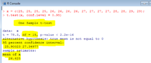
From which we see that the
“95 percent confidence interval”
is
25.90023 to 27.34977
which almost exactly matches our calculation of $[ 25.90038,\ 27.34962 ]$. The difference between our calculation and R’s calculation is due to various round-off errors. The small difference is not important.
Important note for doing the homework.
In Question 10:
the lower limit of the confidence interval is 25.90023
the upper limit of the confidence interval is 27.34977
Question 11. In a sample of $36$ adult male Eastern American Toads the weights in grams are as follows:
x = 25, 25, 25, 25, 26, 26,
26, 26, 27, 27, 27, 27,
28, 28, 29, 29, 25, 25,
25, 25, 26, 26, 26, 26,
27, 27, 27, 27, 28, 28,
29, 29, 28, 28, 29, 29
With respect to calculating the 99% confidence interval for $\mu_x$ find:
(a) the degrees of freedom
(b) the standard error SE
(c) the margin of error MOE
(d) the lower limit of the 99% confidence interval for $\mu_x$
(e) the upper limit of the 99% confidence interval for $\mu_x$
Answer to Question 11.
Video solution to Question 11 showing how to use R
The following R commands were used in the above video.
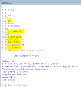
 x = c(25, 25, 25, 25, 26, 26,
26, 26, 27, 27, 27, 27,
28, 28, 29, 29, 25, 25,
25, 25, 26, 26, 26, 26,
27, 27, 27, 27, 28, 28,
29, 29, 28, 28, 29, 29);
x;
sd(x);
sd(x)/sqrt(36);
2.724*(sd(x)/sqrt(36));
mean(x);
26.83333 - 0.6374504;
26.83333 + 0.6374504;
# End of Script
The following R script solves this entire Question.
Note. Some of the results output by the following R script will be slightly different than the results we got in the video using the R commands shown above. This is because in the video we used the t-distribution look-up table to find $t_*$ and in the following R script we have R directly calculate $t_*$. The difference between the two values is insignificant.
x = c(25, 25, 25, 25, 26, 26,
26, 26, 27, 27, 27, 27,
28, 28, 29, 29, 25, 25,
25, 25, 26, 26, 26, 26,
27, 27, 27, 27, 28, 28,
29, 29, 28, 28, 29, 29);
CI = 0.99;
#------- no user input needed below this line ---
n =length(x)
df = n-1
SE = sd(x)/sqrt(n)
t_star = qt( (1 - CI)/2, df, lower.tail = FALSE);
MOE = t_star * SE
LowerLimit_CI = mean(x) - MOE
UpperLimit_CI = mean(x) + MOE
CI
n
df
t_star
SE
MOE
LowerLimit_CI
UpperLimit_CI
t.test(x, conf.level = CI)
# End of Script
R outputs the answers to Question 11: