The following 8 videos (run times vary from 2 to 8 minutes) will help you with your Blackboard homework on this unit.
Please scroll down past these homework videos for an in depth explanation of
Hypothesis Testing & P-values.
Question 2 and 3.
10. Hypothesis Testing: p-values, Exact Binomial Test, Simple one-sided claims about proportions
See Questions 4, 5, and 6, towards the bottom of this page for R scripts to calculate the p-value and a barplot for simple claims about proportions.
There are 2 videos at the end of Question 1 below.
A hypothesis is a claim about a population.
Examples of hypotheses:
- Claim: more than 60% of students like math.
- Claim: the mean weight of cats is less than 9 pounds
We test a claim by taking a sample from the population. If the data from the sample agrees with (or supports) the claim, we say the data provides evidence that the claim is true.
- Claim: more than 60% of students like math. $\rho > 60\%$
Data: If in a sample of 10 students 8 of them like math, the sample supports the claim because $\dfrac{8}{10} = 80\% > 60\%$. If 9 of the 10 liked math, the sample would provide even stronger support because 90% > 80% > 60%. If 6 of the 10 liked math, that data doesn’t support the claim since $\dfrac{6}{10} = 60\%$ is not more than 60%. - Claim: the mean weight of cats is less than 9 pounds. $\mu < 9 \text{ pounds }$
Data: If in a sample of 30 cats the mean weight was 8 pounds, the sample supports the claim because 8 pounds < 9 pounds. If in that sample the mean weight was 6 pounds, it would provide even stronger support of the claim because 6 pounds < 8 pounds < 9 pounds.
If the data from the sample supports the claim we can conduct a formal hypothesis test to determine if the sample provides statistically significant evidence that the claim is true.
After Question 7 (below) is a section on how to report the results of a hypothesis test.
p-value method of hypothesis testing
The p-value concept is difficult to understand at first. My suggestion is to read these definitions and descriptions. Then read through the first two or three Questions and their solutions. Then read these definitions again.
Definition. The sample used in the hypothesis test is called the test-sample.
Definition. The p-value is the maximum probability of getting a sample that provides as much support for the claim as the test-sample if we assume that the claim is false.
Note. “as much support” means the same or stronger support.
So, if the p-value is small, it would be very unlikely for us to get a sample which provides as much support for the claim being true, as the test-sample does, if the claim were false. So, if the p-value is small, the test-sample provides good evidence that the claim wasn’t false. So, a small p-value indicates the test-sample should be considered significant (strong) evidence that the claim is true.
WARNING!!! When we calculate a p-value it is with respect to a mathematical model of the “experiment”. The better the model represents the experimental design, the sampling method, etc., the more relevant will be the p-value. Think about it. Unless the model faithfully represents the experiment, the p-value we calculate will tell us nothing meaningful. For more on this, please read the section, in Question 1 below, called: Important aside about mathematical models.
General algorithm to calculate the p-value:
If the claim is false, the maximum probability of getting a sample which supports the claim happens if the claim is false by the smallest amount possible. Think: little lies are difficult to detect.
So, to calculate the p-value we assume the claim is false by the smallest amount possible and then we calculate the probability of getting a sample that provides as much support as the test-sample.
How small does the p-value have to be in order for it indicate that the test-sample provides significant (strong) evidence that the claim is true?
Definition. If the p-value is smaller than a number called the level of significance, denoted $\alpha$, we say the sample provides statistically significant (strong) evidence that the claim is true.
Unless otherwise noted, in these notes we will always assume that $\alpha = 0.05$ as that is the most common value for $\alpha$.
Type I and type II errors
Type I and type II errors. The definition of the p-value is often given in terms of a concept called a type I error. A type I error is when a false claim is accepted as true. A type II error is when a true claim is rejected as false 1.
We can define the p-value as: the maximum probability of making type I error, if we are willing to accept the claim as true whenever we get a sample that provides as much support as the test-sample.
Important notes about p-values
- Since p-values are a probability we always have $0 \leq \text{ p-value } \leq 1$.
- A small p-value doesn’t mean the claim is true, or even likely to be true.
- A large p-value means the data in the sample should not be reported as evidence of the claim being true.
The p-value method of hypothesis testing is probably the most common way to test a claim. It also is probably the most misunderstood concept in statistics.
The best way to understand the concept of a p-value is to learn how to calculate the p-value for a simple claim where the mathematics is not too difficult: the exact binomial test (see below). Other types of claims will have more complicated ways of calculating the p-value, but the meaning of the p-value doesn’t change.
P-value method of hypothesis testing for simple one-sided claims about a proportion.
The Exact Binomial Test
A simple one-sided claim about a proportion is a claim that a proportion is greater than some percent or less than some percent.
The symbol for proportion is $\rho$.
The name of the hypothesis test that we use for this situation is “the exact binomial test“. Binomial because we use the binomial distribution. Exact because we don’t approximate the binomial distribution by a continuous distribution.
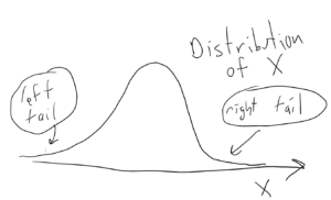
Note. Generally speaking, we test one-sided claims with one-tailed tests. The term “one-tailed” comes from the p-value being the area in one of the “tails” of the distribution. See Figures below and the Figures accompanying the answers to Questions 1 through 6.

Question 1.
Using the p-value method of hypothesis testing test the following claim at the $\alpha = 0.05$ significance level.
- Claim: More than 60% of students are STEM majors.
- Data: In a sample of 10 students 8 of them are STEM majors.
Answer to Question 1. (Also, see video below).
Let:
- $n = $ the size of our sample, so $n = 10$.
- $X = $ the random variable that counts how many of the students in such samples ($n = 10$) are stem majors. $X(\text{our sample}) = 8$
- $\rho = $ “the true proportion of students in the population who are STEM majors”.
The sample’s proportion $\hat{p}$ of STEM majors is $$\hat{p} = \dfrac{X(\text{our sample})}{n} = \dfrac{8}{10} = 80\%$$ which supports our claim because $80\% > 60\%$.
Since the sample supports the claim, we conduct the hypothesis test and calculate the p-value.
In a formal hypothesis test we write the alternative and null hypotheses at the start of the problem. For us, $H_A$ (the alternative hypothesis) will always be the claim and $H_0$ (the null hypothesis) will always be the assumption for the parameters that we will use for our p-value calculation (basically that the claim is false in the smallest way possible):
$\text{(claim) } \ H_A: \rho > 60\%$
$\text{(null) } \ H_0: \rho = 60\%$
Important aside about mathematical models. For simple claims about a proportions, like in Question 1, we model the sampling process as a Bernoulli process having a binomial distribution. When we calculate a p-value it is with respect to the model, not to the actual experiment. The closer the experimental design is is to the model, the more relevant will be the p-value. Think about it. Suppose we have some real-life claim that we are testing. To save money, we could just make up the data and calculate the p-value; or we could collect the data in a sloppy manner, or make a mess of the data in a million ways; but what would a p-value based on such data tell us about the real world? Absolutely nothing.
To calculate the p-value we assume the claim is false by the smallest amount possible and then we calculate the probability of getting a sample that provides as much support as the test-sample.
$X(\text{test-sample}) = 8$ so samples that provide as much support are samples which satisfy $X = 8, 9$, or $10$.
So,
$$\text{p-value} = P(X \geq 8 \ \mid \rho = 60\%)$$
Notation. $P(X \geq 8 \ \mid \rho = 60\%)$ means:
$P(X \geq 8)$ assuming that $\rho = 60\%$
Note. The assumption that $\rho = 60\%$ is the null hypothesis $H_0$. Also, see footnote 2 on $P(A\mid B)$ and Conditional Probability.
As mentioned above, we model our claim and the sampling process as being a Bernoulli process having a binomial distribution with n = 10 and $\rho = 60\%$. Other types of claims and sampling methods will have different mathematical models and involve different types of distributions.
Recall the binomial distribution formula:
$$P(X = r) = nCr\ \rho^r \ (1 – \rho)^{n-r}$$
Substituting in $n = 10$ and $\rho = 60\%$ we finally, actually calculate the p-value:
$\text{p-value} = P(X \geq 8 \ \mid \rho = 60\%)$
$ = P(X = 8) + P(X=9) + P(X= 10) $
$ = 10C8\ (60\%)^8 \ (40\%)^{2} $
$+ 10C9\ (60\%)^9 \ (40\%)^{1} $
$+ 10C10\ (60\%)^{10} \ (40\%)^{0}$
$=0.1209324 + 0.04031078 + 0.006046618$
$ = 0.1672898$
So, the p-value = 0.1672898.
Statistical significance. If the p-value is LESS THAN the significance level $\alpha$ we can report:
- the sample provides statistically significant evidence that the claim is true, or
- the result of the study is statistically significant.
Result. Since the
(p-value = .1672898) > ($\alpha = .05$)
the sample doesn’t provide statistically significant evidence that the claim is true (at the $\alpha = 0.05$ significance level).
Note. In the above calculation, $ P(X = 8) + P(X=9) + P(X= 10) $ are all done with the assumption that $\rho = 60\%$.
Extremely important geometric interpretation of the p-value
See barplot Figure below
Here is the probability density barplot corresponding to the p-value calculated in Question 1, above:
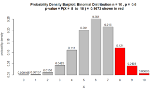
Figure for Question 1. The p-value is the area of the red bars.
For many statisticians, the above Figure is what explains the p-value. As the data from the sample provides more support, the p-value, which is the area of the red bars, decreases. See, for example, Question 2 below.
Note about the above barplot. The heights of the bars are probability densities and the areas of the bars are probabilities. Area = width $\times$ height. Since the bars’ widths are 1, the area of the bars are numerically equivalent to their height. In other words, the numbers on top of the bars are also probabilities. So, for example $P(X=8) = 0.121$.
So, we’ve finished Question 1.
Video showing how to solve Question 1 above (9:35):
Video for Question 1.
Continuation of above video showing solution to Question 2 below (3:34).
Video for Question 1 and 2 showing barplot.
Question 2: Redo the hypothesis test from Question 1, if $X(\text{our sample})$ had been 9, instead of 8. As in Question 1, the sample size is $n =10$ and the level of significance to be used is $\alpha = 0.05$.
Answer to Question 2:
- $n = $ the size of our sample, so $n = 10$.
- $X = $ the random variable that counts how many of the students in such samples are stem majors. $X(\text{our sample}) = 9$
- $\rho = $ “the true proportion of students in the population who are STEM majors”.
The sample’s proportion $\hat{p}$ of STEM majors is $$\hat{p} = \dfrac{X(\text{our sample})}{n} = \dfrac{9}{10} = 90\%$$ which supports our claim because $80\% > 60\%$.
$\text{(claim) } \ H_A: \rho > 60\%$
$\text{(null) } \ H_0: \rho = 60\%$
$\text{p-value} = P(X \geq 9 \ \mid \rho = 60\%)$
$ = P(X=9) + P(X= 10) $
$+ 10C9\ (60\%)^9 \ (40\%)^{1} $
$+ 10C10\ (60\%)^{10} \ (40\%)^{0}$
$= 0.04031078 + 0.006046618$
$ = 0.0463574$
which indicates statistical significance because 0.0463574 < 0.05. Also, see Figure below.
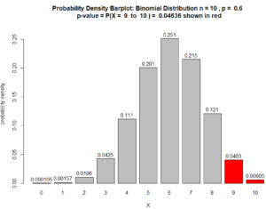
Figure for Question 2. The p-value is the area of the red bars.
Question 3.
Using the p-value method of hypothesis testing test the following claim at the $\alpha = 0.05$ significance level.
- Claim: Less than 60% of students are STEM majors.
- Data: In a sample of 10 students 2 of them are STEM majors.
Answer to Question 3.
- $n = $ the size of our sample, so $n = 10$.
- $X = $ the random variable that counts how many of the students in such samples are stem majors. $X(\text{our sample}) = 2$
- $\rho = $ “the true proportion of students in the population who are STEM majors”.
The sample’s proportion $\hat{p}$ of STEM majors is $$\hat{p} = \dfrac{X(\text{our sample})}{n} = \dfrac{2}{10} = 20\%$$ which supports our claim because $20\% < 60\%$.
$\text{(claim) } \ H_A: \rho < 60\%$
$\text{(null) } \ H_0: \rho = 60\%$
$\text{p-value} = P(X \leq 2 \ \mid \rho = 60\%)$
$ = P(X=0) + P(X= 1) + P(X= 2) $
$+ 10C0\ (60\%)^0 \ (40\%)^{10} $
$+ 10C1\ (60\%)^1 \ (40\%)^{9}$
$+ 10C2\ (60\%)^2\ (40\%)^{8}$
$= 0.0001048576 + 0.001572864 + 0.010616832$
$ = 0.01229$
which indicates statistical significance because the
(p-value = .01229) < ($\alpha = 0.05$)
Also, see Figure below.
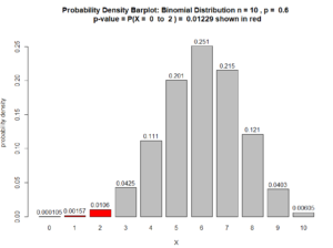
Figure for Question 3. The p-value is the area of the red bars.
Question 4.
Using the p-value method of hypothesis testing test the following claim at the $\alpha = 0.05$ significance level.
- Claim: Less than 49% of children play baseball.
- Data: In a sample of 12 children 3 of them play baseball.
Answer to Question 4.
- $n = $ the size of our sample, so $n = 12$.
- $X = $ the random variable that counts how many of the children in such samples are baseball players. $X(\text{our sample}) = 3$
- $\rho = $ “the true proportion of children in the population who play baseball”.
The sample’s proportion $\hat{p}$ of baseball players is $$\hat{p} = \dfrac{X(\text{our sample})}{n} = \dfrac{3}{12} = 25\%$$ which supports our claim because $25\% < 49\%$.
$\text{(claim) } \ H_A: \rho < 49\%$
$\text{(null) } \ H_0: \rho = 49\%$
$\text{p-value} = P(X \leq 3 \ \mid \rho = 49\%)$
$ = P(X=0) + P(X= 1) + P(X= 2) + P(X=3) $
$+ 12C0\ (49\%)^0 \ (51\%)^{12} $
$+ 12C1\ (49\%)^1 \ (51\%)^{11}$
$+ 10C2\ (49\%)^2\ (51\%)^{10}$
$+ 10C3\ (49\%)^3\ (51\%)^{9}$
$= 0.000309629344375621 $
$+ 0.00356984420574246 $
$+ 0.0188641767342666$
$+ 0.0604146836587622$
$ = 0.08316$
which indicates NO statistical significance because the
(p-value = .08316) > ($\alpha = 0.05$)
Also, see Figure below.
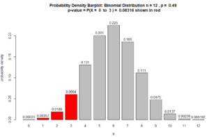
Figure for Question 4. The p-value is the area of the red bars.
Here is the R script used to create the above barplot.
# Simple one-sided claim about proportion p-value barplot
n = 12       # sample size
p = 0.49     # null hypothesis
r_start = 0  # P(X = r_start to r_end)
r_end = 3
#------------------------------------------------
# No need to modify any lines below here
#------------------------------------------------
data = dbinom(x=0:n,size=n, prob=p)
names(data) = 0:n
cols = rep("grey", n + 1)
cols[(r_start + 1): (r_end + 1) ] = "red"
TotalProb = sum(dbinom(x= r_start:r_end,size=n, prob=p))
TotalProbSig = signif(TotalProb, 4)  # use 3 significant digits
titleString = paste("Probability Density Barplot: Binomial Distribution n =" ,n, ", p = ", p,
  "\n p-value = P(X = ", r_start, " to ", r_end, ") = ", TotalProbSig , "shown in red");
b = barplot(data, col = cols, main = titleString ,
xlab = "X", ylab = "probability density", ylim = c(0, 1.1*max(data)))
#------------------------------------------------
barHeights = dbinom(0:n, n, p)
barHeightSig = signif(dbinom(0:n, n, p),3);
#------------------------------------------------
toString(dbinom(0:n, n, p))
text(b,barHeights , labels= barHeightSig , adj=c(0.5, -0.5))
# End of R script
The above script also outputs the distribution of $X$ to the “R Console” window:
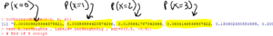
Question 5.
Using the p-value method of hypothesis testing test the following claim at the $\alpha = 0.05$ significance level.
- Claim: More than 55% of children play baseball.
- Data: In a sample of 12 children 10 of them play baseball.
Answer to Question 5.
- $n = $ the size of our sample, so $n = 12$.
- $X = $ the random variable that counts how many of the children in such samples are baseball players. $X(\text{our sample}) = 10$
- $\rho = $ “the true proportion of children in the population who play baseball”.
The sample’s proportion $\hat{p}$ of baseball players is $$\hat{p} = \dfrac{X(\text{our sample})}{n} = \dfrac{10}{12} = 83.3\%$$ which supports our claim because $83.3\% > 55\%$.
$\text{(claim) } \ H_A: \rho > 55\%$
$\text{(null) } \ H_0: \rho = 55\%$
$\text{p-value} = P(X \geq 10 \ \mid \rho = 55\%)$
$ = P(X=10) + P(X= 11) + P(X= 12) $
$+ 12C10\ (55\%)^{10} \ (45\%)^{2} $
$+ 12C11\ (55\%)^{11} \ (45\%)^{1}$
$+ 12C12\ (55\%)^{12}\ (45\%)^{0}$
$= 0.0338528984172231$
$+ 0.00752286631493849$
$+ 0.000766217865410401$
$ = 0.04214$
which indicates the sample provides statistically significant evidence that the claim is true because the
(p-value = .04214) < ($\alpha = 0.05$)
Also, see Figure below.
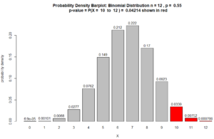
Figure for Question 5. The p-value is the area of the red bars.
Here is the R script used to create the above barplot.
# Simple one-sided claim about proportion p-value barplot
n = 12        # sample size
p = 0.55      # null hypothesis
r_start = 10  # P(X = r_start to r_end)
r_end = n
#------------------------------------------------
# No need to modify any lines below here
#------------------------------------------------
data = dbinom(x=0:n,size=n, prob=p)
names(data) = 0:n
cols = rep("grey", n + 1)
cols[(r_start + 1): (r_end + 1) ] = "red"
TotalProb = sum(dbinom(x= r_start:r_end,size=n, prob=p))
TotalProbSig = signif(TotalProb, 4)  # use 3 significant digits
titleString = paste("Probability Density Barplot: Binomial Distribution n =" ,n, ", p = ", p,
  "\n p-value = P(X = ", r_start, " to ", r_end, ") = ", TotalProbSig , "shown in red");
b = barplot(data, col = cols, main = titleString ,
xlab = "X", ylab = "probability density", ylim = c(0, 1.1*max(data)))
#------------------------------------------------
barHeights = dbinom(0:n, n, p)
barHeightSig = signif(dbinom(0:n, n, p),3);
#------------------------------------------------
toString(dbinom(0:n, n, p))
text(b,barHeights , labels= barHeightSig , adj=c(0.5, -0.5))
# End of R script
The above script also outputs the distribution of $X$ to the “R Console” window:
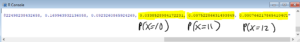
Question 6.
Using the p-value method of hypothesis testing test the following claim at the $\alpha = 0.05$ significance level.
- Claim: More than 51% of children like chocolate.
- Data: In a sample of 200 children 115 of them like chocolate.
Answer to Question 6.
- $n = $ the size of our sample, so $n = 200$.
- $X = $ the random variable that counts how many of the children in such samples like chocolate. $X(\text{our sample}) = 115$
- $\rho = $ “the true proportion of children that like chocolate”.
The sample’s proportion $\hat{p}$ of children who like chocolate is $$\hat{p} = \dfrac{X(\text{our sample})}{n} = \dfrac{115}{200} = 57.5\%$$ which supports our claim because $57.5\% > 51\%$.
$\text{(claim) } \ H_A: \rho > 51\%$
$\text{(null) } \ H_0: \rho = 51\%$
(The following calculation was too long to be done by hand. So I used R.)
$\text{p-value} = P(X \geq 115 \ \mid \rho = 51\%)$
$ = P(X=115) + P(X= 116) + \cdots + P(X= 200) $
$+ 200C115\ (51\%)^{115} \ (49\%)^{85} $
$+ 200C116\ (51\%)^{116} \ (49\%)^{84}$
$\vdots$
$+ 200C200\ (51\%)^{200}\ (49\%)^{0}$
$= 0.010427568 $
$+ 0.007952763$
$\vdots$
$+ 3.266143\times 10^{-59}$
$ = 0.0383$
which indicates the sample provides statistically significant evidence that the claim is true because the
(p-value = .0383) < ($\alpha = .05$)
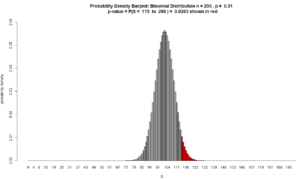
Figure for Question 6. The p-value is the area of the red bars.
Here is the R script used to create the above barplot. Since the bars are very thin, if we put numbers on top of them, the result will be a mess. So, this script omits the numbers on top of the bars.
# Simple one-sided claim about proportion p-value barplot (no numbers on bars)
n = 200        # sample size
p = 0.51       # null hypothesis
r_start = 115  # P(X = r_start to r_end)
r_end = 200
#------------------------------------------------
# No need to modify any lines below here
#------------------------------------------------
data = dbinom(x=0:n,size=n, prob=p)
names(data) = 0:n
cols = rep("grey", n + 1)
cols[(r_start + 1): (r_end + 1) ] = "red"
TotalProb = sum(dbinom(x= r_start:r_end,size=n, prob=p))
TotalProbSig = signif(TotalProb, 4)  # use 3 significant digits
titleString = paste("Probability Density Barplot: Binomial Distribution n =" ,n, ", p = ", p,
  "\n p-value = P(X = ", r_start, " to ", r_end, ") = ", TotalProbSig , "shown in red");
b = barplot(data, col = cols, main = titleString ,
xlab = "X", ylab = "probability density", ylim = c(0, 1.1*max(data)))
#------------------------------------------------
barHeights = dbinom(0:n, n, p)
barHeightSig = signif(dbinom(0:n, n, p),3);
#------------------------------------------------
# End of R script
If we just want to calculate the p-value, the script is much simpler:
# Simple one-sided claim about proportion p-value
n = 200       # sample size
p = 0.51      # null hypothesis
r_start = 115 # P(X = r_start to r_end)
r_end = 200
#------------------------------------------------
# No need to modify any lines below here
#------------------------------------------------
"p-value";
sum(dbinom(x= r_start:r_end,size=n, prob=p));
#------------------------------------------------
# End of R script
Question 7.
Using the p-value method of hypothesis testing test the following claim at the $\alpha = 0.05$ significance level.
- Claim: More than 51% of children like chocolate.
- Data: In a sample of 200 children 100 of them like chocolate.
Answer to Question 7.
- $n = $ the size of our sample, so $n = 200$.
- $X = $ the random variable that counts how many of the children in such samples like chocolate. $X(\text{our sample}) = 100$
- $\rho = $ “the true proportion of children that like chocolate”.
The sample’s proportion $\hat{p}$ of children who like chocolate is $$\hat{p} = \dfrac{X(\text{our sample})}{n} = \dfrac{100}{200} = 50\%$$ which doesn’t support our claim.
The data is contrary to the claim, so we don’t have to calculate the p-value.
End of Question 7.
How to report these results in a scientific paper.
Each journal has its own style for how authors should report their results.
If the sample provided statistical significance, like in Question 6, the authors might write something like:
More than 51% of children like chocolate (p = .0383, exact binomial test).
or
In our survey of 200 children, 57.5% liked chocolate, suggesting more than 51% of children like chocolate (p = .0308, exact binomial test).
The author’s won’t say they did a hypothesis test. They will often state the claim as if it were a fact (even though it isn’t). When they put the p-value they typically leave off the leading zero, so 0.0383 becomes .0383. Also, rather than write p-value, authors typically just write p. The authors won’t usually say that the results are statistically significant: the p-value being less than 0.05 indicates that. Finally, authors should name the type of hypothesis test that they used. In these examples the exact binomial test was used.
If the sample failed to provide statistical significance, for example, if in Question 6 we had $X = 104$, so that $\hat{p} = \dfrac{104}{200} = 52\%$, the p-value would be:
$$\text{p-value } = P(X \geq 104 \mid \rho = 51\%) = .4162$$
If the authors wanted to include this inconclusive result in their paper, they might write something like:
As to the belief that more than 51% of children like chocolate: in our survey of 200 children, 52% said they liked chocolate, which not statistically significant (p = .4162, exact binomial test).
or
Based on our experiences with children, we expected that more than 51% of children would like chocolate: in our survey of 200 children, 52% said they liked chocolate, however this was not statistically significant (exact binomial test).
If the sample provided evidence contrary to the claim, like in Question 7 where we had $X = 100$ so that $\hat{p} = \dfrac{100}{200} = 50\%$ we wouldn’t bother to calculate the p-value (since the sample doesn’t support the claim).
It the authors wanted to include this contrary result, the authors might write something like:
We had thought that more than 51% of children liked chocolate. However, when we surveyed 200 children we found that only 50% said they liked chocolate.
An interesting way to think about the p-value.
- In some sense, the p-value measures how gullible you need to be in order to accept the claim as true based on the data in a sample. So, a smaller p-value indicates you’d need to be less gullible to accept the claim.
How a p-value should be used in the real world
- If the p-value is small, your doubts about the claim being true should be based more on the experimental design, or on an improperly chosen model, or that the authors used the wrong type of hypothesis test; rather than on things like the sample size being too small, or that, due to chance, getting a misleading sample. Note. A small sample size will often result in a large p-value.
- A small p-value doesn’t mean that the claim is true, or is even likely to be true.
- A large p-value doesn’t mean the claim is false.
- A large p-value means the data in the sample should not be presented as evidence of the claim being true.
- Different scientific fields will use different levels of significance to determine if the p-value is small or large, and whether the study can be reported as being “statistically significant”. In these notes we will always use a level of significance of $\alpha = 0.05$ because that is the most commonly used value.
Footnotes:
- Type I and Type II Errors
If we have to decide whether to accept a claim as true, there are two ways we could make a mistake or error.
- Type I Error. A type I error is when a false claim is accepted as true.
Type I errors are made by people who are too trusting and gullible. - Type II Error. A type II error is when we fail to accept a true claim.
Type II errors are made by people who are too cynical.
Obviously we would like to minimize the likelihood of making both types of errors. Unfortunately, if we try to minimize the chances of making a type I error, we need to be more cynical, and that will increase the likelihood of making a type II error. If we try to minimize the chances of making a type II error, we need to be more trusting, and that will increase the likelihood of making a type I error. The only way we can decrease the probability of making both a type I and a type II error is by collecting a larger sample.
- Type I Error. A type I error is when a false claim is accepted as true.
- Notation $P(A \mid B)$
$P(A \mid B)$ is read as the “probability of A assuming B”.
Example. Suppose $X$ is a binomally distributed random variable with $n = 10$. If we write
$$P(X = 8 \mid \rho = 60\%)$$
what we mean is
“the probability that $X = 8$ assuming that $\rho = 60\%$”.
Applying the binomial distribution formula we get:
$P(X = 8 \mid \rho = 60\%)$
$= 10C8\, \rho^8 (1 – \rho)^2$
$= 10C8\, (.60)^8 (.40)^2 $
$= 0.1209324$Same example continued. Since $n = 10$ we have:
$$P(X \geq 9 \mid \rho = 60\%) = P(X = 9 \mid \rho = 60\%) + P(X = 10 \mid \rho = 60\%)$$
However, the above is a little bit long, so to save space, we might write:
$$P(X \geq 9 \mid \rho = 60\%) = P(X = 9) + P(X = 10)$$
where, in the above, $P(X = 9)$ means $P(X = 9 \mid \rho = 60\%)$ and $P(X = 10)$ means $P(X = 10 \mid \rho = 60\%)$.Conditional probability uses the same notation $P(A \mid B)$.
Definition of conditional probability:
$$P(A \mid B) = \dfrac{P(A \cap B}{P(B)}$$
In words $P(A \mid B) = $ the probability that A occurs if we assume that B occurs. The conditional probability $P(A \mid B)$ is read as the “probability of A given B” or the “probability of A assuming B”.
Example. If S = likes to swim and H = likes to hike, then $P(S \mid H)$ is the probability that a person likes to swim if we know they like to hike. $P(H \mid S)$ is the probability that a person likes to hike if we know they like to swim.
If A and B are independent, then $P(A \mid B) = P(A)$ and $P(B \mid A) = P(B)$.