The following 4 videos (run times are from about 1 to 5 minutes each) will help you with your Blackboard homework on this unit.
Please scroll down past these homework videos for an in-depth explanation of the Central Limit Theorem.
Question 3 (below) on “complements” is a review question. For more details about the complement of a set see our Unit on Set Theory:
https://mccarthymat150.commons.gc.cuny.edu/units-0-4/set-theory/
For an a video that uses the z-transformation to solve a Central Limit Theorem Question, scroll down to Question 4 (below).
Introduction to the Central Limit Theorem (CLT)
Suppose we want to estimate the average weight of ripe, wild blueberries growing on Tom Jones Mountain in New York.

Wild blueberry bushes with ripe blueberries.
Tom Jones Mountain. Harriman State Park, NY.
We can’t pick and weigh all the blueberries. So instead, we collect a sample and find the average (mean) weight of the blueberries in that sample.
Different samples of blueberries will have (slightly) different mean weights.
The distribution of the mean weights of the different samples is an example of a sampling distribution.
The Central Limit Theorem (CLT) tells us that if the sample size $n$ is sufficiently large, that the distribution of the means (of a fixed sample size $n$) will be approximately normal. As $n$ increases, the approximation gets better.
The key thing is this. The original random variable (like the weight) might not be normally distributed, however, if we look at the distribution of the samples’ means, that will be approximately normal, provided $n$ is large enough.
For many applications, if $n \geq 30$, $n$ is considered large enough that the CLT can be applied.
CLT
Suppose we obtain a sample of size $n$ from a population and that $x$ is a random variable on that population. The mean of this sample with respect to the random variable $x$ is given by the formula
$$\bar{x} = \frac{\sum_{i = 1}^{n} x_i}{n} $$
where $x_i$ is the value of $x$ applied to the $i^{th}$ member of the sample.
For a review of $\bar{x}$ see Unit 5.
If we fix $n$, meaning, if we keep the sample size $n$ constant, we can consider $\bar{x}$ to be random variable operating on samples of size $n$ taken from that population.
Central Limit Theorem (CLT). If $\mu_x$ and $\sigma_x$ are the mean and standard deviation of $x$, then
$$\mu_{\bar{x}} = \mu_{x} \ \ \ \ (Equation\ 1)$$
and
$$\sigma_{\bar{x}} = \dfrac{\sigma_{x}}{\sqrt{n}} \ \ \ \ (Equation\ 2)$$
Case 1. If $n$ is large enough, then $\bar{x}$ will be approximately normal.
Case 2. If $x$ is normal, then even if $n$ is small, $\bar{x}$ will be normal.
So, if $n$ is large enough, or if $x$ was normal to begin with, Equations 1 and 2 imply we can write:
$$\bar{x} \sim N\left(\mu_{\bar{x}}, \sigma_{\bar{x}}\right) = N\left(\mu_{x} , \dfrac{\sigma_{x}}{\sqrt{n}} \right)$$
For a proof see Wikipedia: https://en.wikipedia.org/wiki/Central_limit_theorem
Note. If $x$ itself is heavily skewed, meaning the distribution of $x$ is far from being symmetric about its mean, then the “normal approximation” of $\bar{x}$ as being $N\left(\mu_{x} , \dfrac{\sigma_{x}}{\sqrt{n}} \right)$ will not be a very good approximation, unless $n$ is very large, much larger than 30.
Note. When we solve problems we’ll often write that $\bar{x}$ is normally distributed, even if we should write $\bar{x}$ is approximately normally distributed.
CLT Questions
CLT questions are solved the same way normal distribution problems are solved. The only difference is that now $\sigma_{\bar{x}} = \dfrac{\sigma_x}{\sqrt{n}} $.
Question 1.
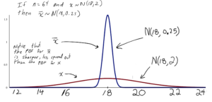
Suppose that the mean height of giraffes is 18 feet and with a standard deviation of 2 feet. If we measure the heights of 64 randomly chosen giraffes, what is the probability the mean height of the giraffes in our sample will be between 18 and 18.5 feet? Let $x$ be the random variable which measures the heights of giraffes.
Solution to Question 1.
Since $n = 64 \geq 30$ the CLT implies that $\bar{x}$ will be approximately normally distributed.
$\mu_{\bar{x}} = \mu_x = 18$
and
$\sigma_{\bar{x}} = \dfrac{\sigma_x}{\sqrt{n}} = \dfrac{2}{\sqrt{64}}$
$= \dfrac{2}{8} = 0.25 $
So $\bar{x} \sim N(18, 0.25)$.
Then, using R, we have:
$P(18 < \bar{x} < 18.5 ) = P(\bar{x} < 18.5) – P(\bar{x} < 18) $
$= \text{pnorm}(18.5, 18, 0.25) – \text{pnorm}(18, 18, 0.25)$
$= 0.9772499 – 0.5$
$= 0.4772499 \ \leftarrow \ \ answer$
Here is the R code that will do the calculation for Question 1:
# Central Limit Theorem Calculation
# P(a < xbar < b)
mux = 18;
sdx = 2;
n = 64;
a = 18;
b = 18.5;
# end of user input
mu_xbar = mux
sd_xbar = sdx/sqrt(n);
pnorm(b,mu_xbar,sd_xbar) - pnorm(a,mu_xbar,sd_xbar);
# End of Script
We can also solve Question 1 without using R.
We can find
$P(18 < \bar{x} < 18.5 )$
by calculating the z-scores and using the z-table. The z-score
$z(x) = \dfrac{x-\mu_x}{\sigma_x}$
becomes
$z(\bar{x}) = \dfrac{\bar{x}-\mu_{\bar{x}}}{\sigma_{\bar{x}}}$.
So:
$z(\bar{x}) = \dfrac{\bar{x}-18}{0.25}$
$z(18) = \dfrac{18-18}{0.25} = 0$
$z(18.5) = \dfrac{18.5-18}{0.25} = \dfrac{0.5}{0.25} =2$
and so:
$P(18 < \bar{x} < 18.5 ) $
$= P(z(18) < z(\bar{x}) < z(18.5)) $
$= P(0 < z < 2.00)$
$= A(2.00) – A(0.00) $
$= .9772 – .5000$
$ = .4772 \ \ \leftarrow \ \ answer$
Question 2.
Suppose that the mean height of giraffes is 18 feet and with a standard deviation of 2 feet. If we measure the heights of 64 randomly chosen giraffes, what is the probability the mean height of the giraffes in our sample will be more than 17.8 feet? Let $x$ be the random variable which measures the heights of giraffes.
Solution to Question 2.
Since $n = 64 \geq 30$ the CLT implies that $\bar{x}$ will be approximately normally distributed.
$\mu_{\bar{x}} = \mu_x = 18$
and
$\sigma_{\bar{x}} = \dfrac{\sigma_x}{\sqrt{n}} = \dfrac{2}{\sqrt{64}}$
$= \dfrac{2}{8} = 0.25 $
So $\bar{x} \sim N(18, 0.25)$.
Then, using R, we have:
$P( \bar{x} > 17.8 ) = 1 – P(\bar{x} < 17.8) $
$= 1 – \text{pnorm}(17.8, 18, 0.25)$
$= 1 – 0.2118554$
$= 0.7881446 \ \leftarrow \ \ answer$
We can also solve Question 2 without using R.
We can also find
$P(\bar{x} > 17.8 )$
by calculating the z-scores and using the z-table. The z-score
$z(x) = \dfrac{x-\mu_x}{\sigma_x}$
becomes
$z(\bar{x}) = \dfrac{\bar{x}-\mu_{\bar{x}}}{\sigma_{\bar{x}}}$.
So:
$z(\bar{x}) = \dfrac{\bar{x}-18}{0.25}$
$z(17.8) = \dfrac{17.8-18}{0.25} = \dfrac{-0.20}{0.25} = -0.80$
and so:
$P(17.8 < \bar{x} ) $
$= P(z(17.5) < z(\bar{x}) ) $
$= P(-2 < z ) $
$= 1 – P(z < -0.80)$
$= 1 – A(-0.80) $
$= 1 – .2119$
$ = 0.7881 \ \ \leftarrow \ \ answer$
Question 3.
Suppose that the mean weight of wild blueberries is 0.3 grams (g) with a standard deviation of 0.06 g. What is the probability that the total weight of 36 wild blueberries will be less than 11 g? Let $x$ be the random variable which measures the weights of wild blueberries.
Solution to Question 3.
The total weight of the blueberries in a sample being less than 11 grams is equivalent to the mean weight of the blueberries in the sample being less than $\dfrac{11 }{36} \ \text{grams}$ because
$\text{the mean weight of blueberries in sample} = \dfrac{\text{total weight of sample}}{\text{size of sample}} $
Since $n = 36 \geq 30$ the CLT implies that $\bar{x}$ will be approximately normally distributed.
$\mu_{\bar{x}} = \mu_x = 0.3$
and
$\sigma_{\bar{x}} = \dfrac{\sigma_x}{\sqrt{n}} = \dfrac{0.06}{\sqrt{36}}$
$= \dfrac{0.06}{6} = 0.01$
So $\bar{x} \sim N(0.3, 0.01)$ measured in grams.
Then, using R, we have:
$P( \bar{x} < 11/36) $
$= \text{pnorm}(11/36, 0.3, 0.01)$
$= 0.7107426 \ \leftarrow \ \ answer$
Note. In the above, I put 11/6 directly in R’s pnorm function rather than the decimal approximation of 11/6.
We can also solve Question 3 without using R.
We can also find
$P(\bar{x} < 11/36)$
by calculating the z-scores and using the z-table.
We have to use decimals with the z-table.
$\dfrac{11}{36} = 0.3055556$ so $P(\bar{x} < 11/36) = P(\bar{x} < 0.3055556)$
The z-score
$z(x) = \dfrac{x-\mu_x}{\sigma_x}$
becomes
$z(\bar{x}) = \dfrac{\bar{x}-\mu_{\bar{x}}}{\sigma_{\bar{x}}}$.
So:
$z(\bar{x}) = \dfrac{\bar{x}-0.3}{0.01}$
$z(0.3055556) = \dfrac{0.3055556 – 0.3}{0.01} $
$= \dfrac{0.0055556}{0.01} = 0.55556 \approx 0.56$
and so:
$P( \bar{x} < 0.3055556) $
$= P(z(\bar{x}) < z( 0.3055556)) $
$= P(z< 0.56 ) $
$= A(0.56) $
$= .7123 \ \ \leftarrow \ \ answer$
The answer we get using the z-table is a little different than the answer we get using R because we have to round of some of the numbers to use the z-table. R’s answer is the more accurate one.
Question 4.
Suppose the mean age of trees in a forest is 50 years with a standard deviation of 20 years. Find the probability that a random sample of 36 trees from that forest will have a mean age of between 49 and 51 years.
Solution to Question 4.
See video.
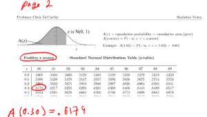
Using the z-table to find A(0.30) and A(-0.30). For details see unit 12 on the standard normal distribution.

Question 5. (This question is about total weight, but is solved using the CLT)
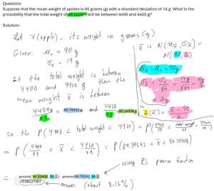
Suppose the mean weight of apples is 90 grams (g) with a standard deviation of 14 g. What is the probability that the total weight of 49 apples will be between 4400 g and 4420 g?
Solution to Question 5.
The trick to solving this problem is to divide the total weight of the 49 apples by 49 to get the mean weight of those 49 apples. This allows us to use the Central Limit Theorem (CLT). To use the CLT we need to find the mean and standard deviation of $\bar{x}$: $\mu_{\bar{x}} = \mu_{x} = 90\ g\ $ and $\sigma_{\bar{x}} = \frac{\sigma_{x}}{\sqrt{n}} = \frac{14}{\sqrt{49}} = \frac{14}{7} = 2\ g$ where $x(\text{an apple}) = $ its weight in grams. See the image immediately below for the details of how I solve Question 5:
Comparing $\mathbf{x}$ and $\mathbf{\bar{x}}$
As $n$ increases the standard deviation of $\bar{x}$ decreases. As a result, as $n$ increases it becomes more likely that a sample’s mean will be close to the population mean.
The following Figure illustrates this by comparing the PDF’s of $x$ and $\bar{x}$. Notice that the PDF of $\bar{x}$ has a sharper peak.